Introduction to Decision Tree in Supervised Learning
Introduction
Decision Tree is one of the Supervised Learning Algorithm in Machine Learning. Supervised Learning algorithms are the one that learn to associate some input with some output, given a training set of examples of input x and output y. Practically the output y may be difficult to collect automatically and must be provided by a human “supervisor”, also called as “Data Labelling”. There are variety of algorithms available in Supervised Learning, broadly classified as; “Probablistic” and “Non Probablistic”. Decision Tree algorithm falls in “Non-Probablistic” category similar to k-nearest neighbors algorithm.
Decision Tree algorithm breaks the input space into regions and has separate parameters for each region. Decision Trees can be used both for classification and regression purposes. A decision tree can be imagined as a structure that includes a root node, branches, and leaf nodes. Each internal node denotes a test on an attribute, each branch denotes the outcome of a test, and each leaf node holds a class label. The topmost node in the tree is the root node.
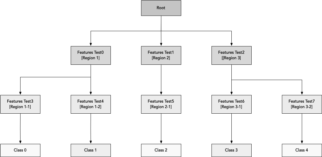
As shown in above diagram, each node of the decision tree is associated with a region in the input space, and internal nodes break that region into one subregion for each child of the node.
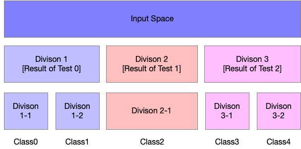
Space is thus subdivided into nonoverlapping regions, with a one-to-one correspondance between leaf nodes and input regions. Each Leaf node usually maps every point in its imput region to the same output. Each Leaf requires atleast one training example to define, so it is not possible for decision tree to learn a function that has more local maxima than the number of training examples.
This algorithm can be considered nonparametric if it is allowed to learn a tree of arbitrary size, but typically decision trees are regularised with size constraints that turn them into parametric models in practice.
Classification And Regression Trees (CART)
In recent days, the decession tree algorithms are called as CART, which stands for Classification and Regression Trees. CART is a term introduced by Leo Breiman in 1984 to refer to Decision Tree algorithms that can be used for classification and regression modeling problems. The CART algorithm provides a foundation for other important algorithms like bagged decision trees, random forest and boosted decision trees.
Decision Trees are prefered for its stability, reliability and explainability. These algorithms are very useful when computational resources are constrained.
Terminologies
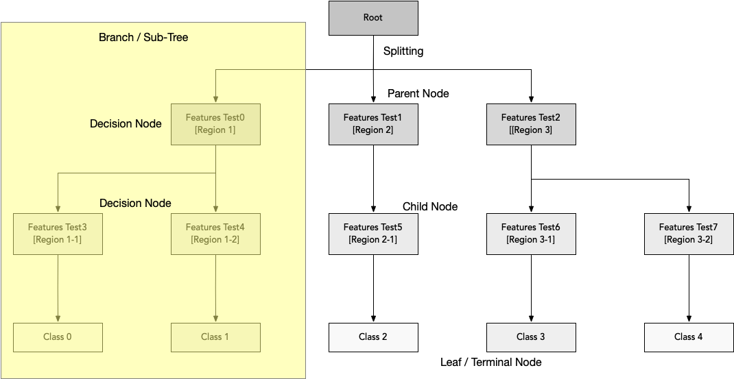
As described earlier, the algorithm will follow a tree like structure in which each internal node represents a test on an attribute, each branch represents the outcome of the test, and each leaf node represents a class lavel. The paths from the root node to leaf node represents the classification rules. Following are the terminologies involved in Decision Tree algorithm:
Root Node: Represents the entire input space.
Splitting: Process of dividing the node into two or more sub-nodes.
Decision Node: The node that gets further divided into different sub-nodes
Leaf or Terminal Node: Nodes that do not split further
Pruning: Process of removing sub-nodes of a decision node. Basically its opposite of Splitting
Branch/Sub-Tree: Sub-section of an entire tree
Parent and Child Node: Node which is divided into sub-nodes is called parent node of the sub-nodes. And the sub-nodes are the children of the parent node.
The algorithm can be simply stated as follows:
- For each attribute in the dataset the algorithm forms a node. The most important attribute is placed at the root node
- For evaluating the task in hand, the algorithm starts at the root node and work its way down the treeby following the corresponding node that meets the condition or decision
- The process continues until a leaf node is reached. The leaf node contains the prediction or the outcome of the tree
Attribute selection measures
As you observed, the primary challenge in decision tree implementation is to identify the attributes that forms the root node and decision node at each level of the tree. This process is known as attributes selection. There are two popular attribute selection measures:
- Information Gain
- Gini Index
Information Gain
The key assumption here is that the attributes or features are categorical. The idea here is to estimate the information contained by each attribute. To understand this better, it important to know the concept called Entropy. Entropy is the measure of uncertainty of a random variable, it characterizes the impurity of an arbitrary collection of examples. The higher the entropy more the information content.
Information gain is a measure of this change in entropy. Information gain computes the difference between entropy before split and average entropy after split of the dataset based on given attribute values. The ID3(Iterative Dichotomiser) decision tree algorithm uses entropy to calculate the information gain. The attribute with the highest information gain is chosen as the splitting attribute at the node. The mathematical formula to compute Entropy is:
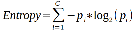
Note: Here c is the number of classes and pi is the probability assocuated with the ith class.
Gini Index
The key assumption here is that the attributes or features are continuous. Gini Index is a metric to measure how often a randomly chosen element would be incorrectly identified. Unlike Information Gain, where the attribute with highest gain is chosen, Gini Index chooses an attribute with lower index.
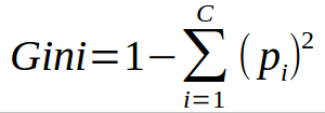
Note: Here c is the number of classes and pi is the probability assocuated with the ith class.
Common Types of Decision Tree Algorithms
- Iterative Dichotomiser 3 (ID3): This algorithm uses Information Gain to decide which attribute is to be used classify the current subset of the data. For each level of the tree, information gain is calculated for the remaining data recursively.
- C4.5: This algorithm is the successor of the ID3 algorithm. This algorithm uses either Information gain or Gain ratio to decide upon the classifying attribute. It is a direct improvement from the ID3 algorithm as it can handle both continuous and missing attribute values.
- CART: It is a dynamic learning algorithm which can produce a regression tree as well as a classification tree depending upon the dependent variable.
Overfitting in Decision Tree
Overfitting is a common problem in almost all supervised learning algorithms. The problem is that the algorithms or models memorised the entire training set resulting in very low training set error but high testing set error. In decision tree, overfitting means the model built many branches due to outliers and irregularities in data. In practice, following two approaches used to avoid overfitting:
- Pre-Pruning: Stops the tree construction bit early. Basically don’t split a node if its goodness measure is below a threshold value. Pratically it is difficult to choose an appropriate stopping point.
- Post-Pruning: In this case the pruning happens after the entire tree is built and you observe overfitting problem. The cross-validation method is used to check the effect of pruning. Using cross-validation date, check whether expanding a node will result in improvement or not. If it shows an improvement, then continue expanding the node otherwise stop expansion (or splitting) and the node converted to terminal node.
Example Decision Tree Notebook
# Importing required libraries

import numpy as np
import pandas as pd
import matplotlib.pyplot as plt
import seaborn as sns
import warnings

warnings.filterwarnings('ignore')
# Import Car Evaluation Dataset
# Refer https://archive.ics.uci.edu/ml/machine-learning-databases/car/car.names
df = pd.read_csv('https://archive.ics.uci.edu/ml/machine-learning-databases/car/car.data', header=None)
df.shape
(1728, 7)
df.head()
| 0 | 1 | 2 | 3 | 4 | 5 | 6 | |
|---|---|---|---|---|---|---|---|
| 0 | vhigh | vhigh | 2 | 2 | small | low | unacc |
| 1 | vhigh | vhigh | 2 | 2 | small | med | unacc |
| 2 | vhigh | vhigh | 2 | 2 | small | high | unacc |
| 3 | vhigh | vhigh | 2 | 2 | med | low | unacc |
| 4 | vhigh | vhigh | 2 | 2 | med | med | unacc |
# Rename Columns
df.columns = ['buying', 'maint', 'doors', 'persons', 'lug_boot', 'safety', 'class']
df.sample()
| buying | maint | doors | persons | lug_boot | safety | class | |
|---|---|---|---|---|---|---|---|
| 313 | vhigh | med | 5more | 4 | big | med | acc |
# Summary of Data
df.info()
df.describe().T
<class 'pandas.core.frame.DataFrame'>
RangeIndex: 1728 entries, 0 to 1727
Data columns (total 7 columns):
 #   Column    Non-Null Count  Dtype
---  ------    --------------  -----
 0   buying    1728 non-null   object
 1   maint     1728 non-null   object
 2   doors     1728 non-null   object
 3   persons   1728 non-null   object
 4   lug_boot  1728 non-null   object
 5   safety    1728 non-null   object
 6   class     1728 non-null   object
dtypes: object(7)
memory usage: 94.6+ KB
| count | unique | top | freq | |
|---|---|---|---|---|
| buying | 1728 | 4 | low | 432 |
| maint | 1728 | 4 | low | 432 |
| doors | 1728 | 4 | 4 | 432 |
| persons | 1728 | 3 | 4 | 576 |
| lug_boot | 1728 | 3 | small | 576 |
| safety | 1728 | 3 | low | 576 |
| class | 1728 | 4 | unacc | 1210 |
# Frequency Distribution of Attributes
for col in df.columns:
    print(df[col].value_counts())
low      432
vhigh    432
high     432
med      432
Name: buying, dtype: int64
low      432
vhigh    432
high     432
med      432
Name: maint, dtype: int64
4        432
5more    432
3        432
2        432
Name: doors, dtype: int64
4       576
more    576
2       576
Name: persons, dtype: int64
small    576
med      576
big      576
Name: lug_boot, dtype: int64
low     576
high    576
med     576
Name: safety, dtype: int64
unacc    1210
acc       384
good       69
vgood      65
Name: class, dtype: int64
Data Summary
There are 7 attributes in the dataset. All the attributes are of categorical data type.
These are given by buying, maint, doors, persons, lug_boot, safety and class.
class is the target attribute, which has the following values:
- unacc (70%)
- acc (22.22%)
- good (4%)
- vgood (3.8%)
# check missing values in variables
df.isnull().sum()
buying      0
maint       0
doors       0
persons     0
lug_boot    0
safety      0
class       0
dtype: int64
# Split Feature & Target attributes

X = X = df.drop(['class'], axis=1)

y = df['class']
# split X and y into training and testing sets

from sklearn.model_selection import train_test_split

X_train, X_test, y_train, y_test = train_test_split(X, y, test_size = 0.3, random_state = 100)
# Check the shapes of training and testing sets
X_train.shape, y_train.shape, X_test.shape, y_test.shape
((1209, 6), (1209,), (519, 6), (519,))
# Encode the categorical variables
import category_encoders as ce

# encode variables with ordinal encoding
encoder = ce.OrdinalEncoder(cols=['buying', 'maint', 'doors', 'persons', 'lug_boot', 'safety'])

X_train = encoder.fit_transform(X_train)

X_test = encoder.transform(X_test)
X_train.head()
| buying | maint | doors | persons | lug_boot | safety | |
|---|---|---|---|---|---|---|
| 774 | 1 | 1 | 1 | 1 | 1 | 1 |
| 1021 | 2 | 2 | 2 | 1 | 2 | 2 |
| 105 | 3 | 3 | 3 | 1 | 3 | 1 |
| 44 | 3 | 3 | 2 | 2 | 3 | 3 |
| 1374 | 4 | 3 | 4 | 1 | 3 | 1 |
X_test.head()
| buying | maint | doors | persons | lug_boot | safety | |
|---|---|---|---|---|---|---|
| 27 | 3 | 3 | 2 | 3 | 1 | 1 |
| 1156 | 2 | 4 | 4 | 1 | 2 | 2 |
| 1668 | 4 | 1 | 2 | 1 | 2 | 1 |
| 1622 | 4 | 1 | 1 | 3 | 1 | 3 |
| 692 | 1 | 4 | 2 | 2 | 3 | 3 |
# The dataset is now ready for modelling
# import DecisionTreeClassifier
from sklearn.tree import DecisionTreeClassifier

# instantiate the DecisionTreeClassifier model with criterion gini index
clf_gini = DecisionTreeClassifier(criterion='gini', max_depth=3, random_state=0)
# Fit the model
clf_gini.fit(X_train, y_train)
DecisionTreeClassifier(max_depth=3, random_state=0)
# Predict by using Testing set
y_pred_gini = clf_gini.predict(X_test)
from sklearn.metrics import accuracy_score

print('Model accuracy score with criterion gini index: {0:0.4f}'. format(accuracy_score(y_test, y_pred_gini)))
Model accuracy score with criterion gini index: 0.7842
# Let's compare training and test set accuracy to check whether we have overfitting problem
y_pred_train_gini = clf_gini.predict(X_train)
print('Training-set accuracy score: {0:0.4f}'. format(accuracy_score(y_train, y_pred_train_gini)))
Training-set accuracy score: 0.7750
Here, the training-set accuracy score is 0.7750 while the test-set accuracy to be 0.7842. These two values are quite comparable. So, there is no sign of overfitting.
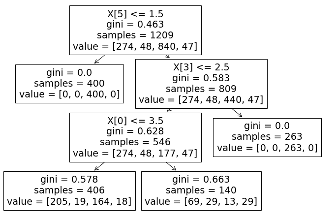
Visualising Decision Tree
plt.figure(figsize=(12,8))

from sklearn import tree

tree.plot_tree(clf_gini.fit(X_train, y_train))
[Text(267.84000000000003, 380.52, 'X[5] <= 1.5\ngini = 0.463\nsamples = 1209\nvalue = [274, 48, 840, 47]'),
 Text(133.92000000000002, 271.8, 'gini = 0.0\nsamples = 400\nvalue = [0, 0, 400, 0]'),
 Text(401.76000000000005, 271.8, 'X[3] <= 2.5\ngini = 0.583\nsamples = 809\nvalue = [274, 48, 440, 47]'),
 Text(267.84000000000003, 163.07999999999998, 'X[0] <= 3.5\ngini = 0.628\nsamples = 546\nvalue = [274, 48, 177, 47]'),
 Text(133.92000000000002, 54.360000000000014, 'gini = 0.578\nsamples = 406\nvalue = [205, 19, 164, 18]'),
 Text(401.76000000000005, 54.360000000000014, 'gini = 0.663\nsamples = 140\nvalue = [69, 29, 13, 29]'),
 Text(535.6800000000001, 163.07999999999998, 'gini = 0.0\nsamples = 263\nvalue = [0, 0, 263, 0]')]
Visualising Decision Tree using Graphwiz
import graphviz
dot_data = tree.export_graphviz(clf_gini, out_file=None,
                              feature_names=X_train.columns,
                              class_names=y_train,
                              filled=True, rounded=True,
                              special_characters=True)

graph = graphviz.Source(dot_data)

graph

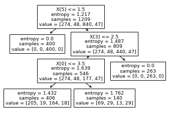
# Decision Tree using Entropy method
clf_en = DecisionTreeClassifier(criterion='entropy', max_depth=3, random_state=0)

# fit the model
clf_en.fit(X_train, y_train)

y_pred_en = clf_en.predict(X_test)
y_pred_train_en = clf_en.predict(X_train)
print('Training-set accuracy score: {0:0.4f}'. format(accuracy_score(y_train, y_pred_train_en)))
print('Model accuracy score with criterion entropy: {0:0.4f}'. format(accuracy_score(y_test, y_pred_en)))
Training-set accuracy score: 0.7750
Model accuracy score with criterion entropy: 0.7842
We can see that the training-set score and test-set score is same as above. The training-set accuracy score is 0.7750 while the test-set accuracy to be 0.7842. These two values are quite comparable. So, there is no sign of overfitting.
# Visalising the Trees
tree.plot_tree(clf_en.fit(X_train, y_train))
[Text(133.92000000000002, 190.26, 'X[5] <= 1.5\nentropy = 1.217\nsamples = 1209\nvalue = [274, 48, 840, 47]'),
 Text(66.96000000000001, 135.9, 'entropy = 0.0\nsamples = 400\nvalue = [0, 0, 400, 0]'),
 Text(200.88000000000002, 135.9, 'X[3] <= 2.5\nentropy = 1.487\nsamples = 809\nvalue = [274, 48, 440, 47]'),
 Text(133.92000000000002, 81.53999999999999, 'X[0] <= 3.5\nentropy = 1.639\nsamples = 546\nvalue = [274, 48, 177, 47]'),
 Text(66.96000000000001, 27.180000000000007, 'entropy = 1.432\nsamples = 406\nvalue = [205, 19, 164, 18]'),
 Text(200.88000000000002, 27.180000000000007, 'entropy = 1.762\nsamples = 140\nvalue = [69, 29, 13, 29]'),
 Text(267.84000000000003, 81.53999999999999, 'entropy = 0.0\nsamples = 263\nvalue = [0, 0, 263, 0]')]
dot_data = tree.export_graphviz(clf_en, out_file=None,
                              feature_names=X_train.columns,
                              class_names=y_train,
                              filled=True, rounded=True,
                              special_characters=True)

graph = graphviz.Source(dot_data)

graph

Now, based on the above analysis we can conclude that our classification model accuracy is very good. Our model is doing a very good job in terms of predicting the class labels.
But, it does not give the underlying distribution of values. Also, it does not tell anything about the type of errors our classifer is making.
Confusion matrix & Classification Report helps us here.
from sklearn.metrics import confusion_matrix,classification_report

cm = confusion_matrix(y_test, y_pred_en)

print('Confusion matrix\n', cm)
print('\nClassification Report\n', classification_report(y_test, y_pred_en))
Confusion matrix
 [[110   0   0   0]
 [ 21   0   0   0]
 [ 73   0 297   0]
 [ 18   0   0   0]]

Classification Report
               precision    recall  f1-score   support

         acc       0.50      1.00      0.66       110
        good       0.00      0.00      0.00        21
       unacc       1.00      0.80      0.89       370
       vgood       0.00      0.00      0.00        18

    accuracy                           0.78       519
   macro avg       0.37      0.45      0.39       519
weighted avg       0.82      0.78      0.78       519
Results and Conclusion
- In the above example, two Decision-Tree Classifier models are built to predict the safety of the care. One model with Gini Index criterion and another with Information Gain (Entropy) criterion. Both the model yields very good performance as indicated by the model accuracy.
- In both the models the accuracy scores of both Training and Testing sets are quite comparable. So, there is no sign of overfitting.
- In both the models, the training-set and test-set accuracy score is the same. It may happen because of small dataset.
- The confusion matrix and classification report shows very good model performance.
Jupyter Notebook Download
Click here to download the notebook
Reference Links
- https://www.geeksforgeeks.org/decision-tree-introduction-example/
- https://www.kaggle.com/prashant111/decision-tree-classifier-tutorial
- Deep Learning by Ian Goodfellow, Yoshua Benigo and Aaron Courville